9
Jan
How to Build, Measure & Control a Superconducting Qubit
By
Remo Marini
When discussing quantum mechanics, everyone inevitably rely on mathematical representations. It is, in fact, the easiest way to describe a system and make predictions, especially given how counterintuitive quantum behavior can sometimes be.
Therefore, it’s common to represent a qubit mathematically as:
\[
\mathrm{qubit} = \alpha\,|0\rangle + \beta\,|1\rangle =
\begin{pmatrix}
\alpha \\
\beta
\end{pmatrix}
\]
which expresses a qubit as a sum (linear superposition) of the two possible states of a bit, 0 and 1. Each basis state is multiplied by a coefficient alpha or beta, respectively, which are complex numbers.
Although this linear algebra formulation looks daunting at first, it actually makes understanding operations on the qubit (and on multiple qubits) extremely simple.
These operations – also called quantum gates – are the core of quantum algorithms and, in this representation, are nothing more than matrices. Applying a transformation to the qubit states is equivalent to multiplying the vector by the matrix. In short, you’ve moved from advanced physics to (a simpler) linear algebra.
To perform any possible operation on a quantum computer, you need a so-called universal set of gates. This means a collection of basic operations (or matrices) that can be combined to create any other operation.
To form a universal gate set, we require the ability to manipulate single qubits arbitrarily (single-qubit gates), and at least one kind of two-qubit gate to create entanglement between qubits.
A few examples of single qubit gates are:
- The NOT gate, which flips |0⟩ to |1⟩ and vice versa, represented in matrix form as
\[
X =
\begin{pmatrix}
0 & 1 \\
1 & 0
\end{pmatrix}
\]
- The Hadamard gate H, which creates an equal superposition of |0⟩ and |1⟩ , given by
\[
H=\frac{1}{\sqrt{2}}
\begin{pmatrix}
1 & 1 \\
1 & -1
\end{pmatrix}
\]
While the most famous two-qubit gate is the controlled-NOT (CNOT) gate:
\[ \mathrm{CNOT} = \begin{pmatrix} 1 & 0 & 0 & 0 \\ 0 & 1 & 0 & 0 \\ 0 & 0 & 0 & 1 \\ 0 & 0 & 1 & 0 \end{pmatrix} \]
which flips the second qubit (target) if and only if the first qubit (control) is |1⟩ , and does nothing otherwise.
This abstract linear algebra view makes it easy to talk about transformations and algorithms by ignoring physical details.
Let us consider one of the simplest set of quantum gates there is:
2 qubits both starting in the |0⟩ state, then applying the Hadamard (H) gate to qubit 1 and subsequently the CNOT gate to both of them.
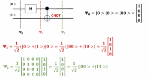
This simple algorithm made of two matrix multiplications has profound physical meaning, it starts from two distinct qubits and entangles them.
” Entanglement can be understood as perfectly correlated randomness. When you measure an entangled qubit, the outcome is unpredictable (randomness), but when you measure its entangled partner, you will always get the same result (perfect correlation). Mathematically it can be written as (this is just one of the four Bell states):
\[
\frac{1}{\sqrt{2}}\left( |00\rangle + |11\rangle \right)
\]
In simple terms, this means if you measure 0 on one qubit, you will also measure 0 on the other. The same applies for the 1 state (you will never see a |01⟩ combination).
This clearly demonstrates why this abstract formulation is so popular—the intricate and seemingly absurd physics of entanglement emerges naturally from a few simple matrix multiplications.
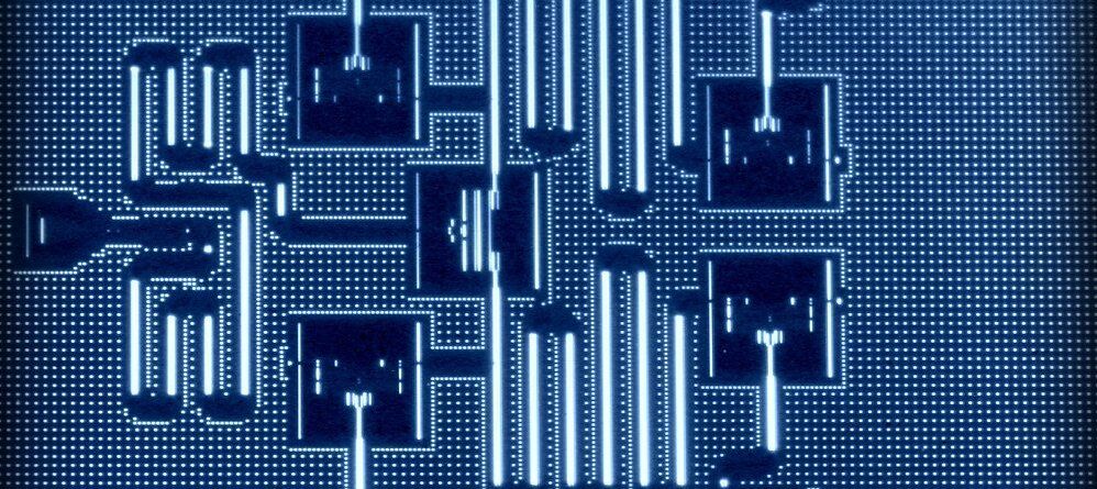
But what is really happening behind the curtains at the hardware level? How do we build a physical qubit and actually perform these gates on a real device? Also how do we measure a qubit? To answer this, we are peeking under the hood of a superconducting quantum computer.
Creating a Superconducting Qubit
Superconducting qubits represent just one approach to building quantum bits. Several other implementations exist, including trapped ions, neutral atoms, photonics, silicon-based qubits, topological qubits, and more.
In principle, any quantum two-level system can serve as a qubit. The fundamental concept involves taking a classical bit with its distinct 0/1 values and encoding it in a quantum system. This quantum encoding provides computational advantages through superposition and entanglement—unique features that arise from the system’s quantum nature.
However, this is not the complete picture. While all of the above is true, a qubit must have certain properties to function properly. We need to be able to prepare it, interact with it, and read it. These requirements are formalized in the DiVincenzo criteria, which include [1]:
- Scalable physical qubits: a large, well-defined two-level system that can be extended to many qubits.
- Initialization: a reliable way to start qubits in a known state (usually ∣0⟩).
- Long coherence times: the qubits must preserve superpositions long enough to perform computations.
- Universal set of gates: the ability to perform arbitrary single-qubit operations and at least one entangling two-qubit operation.
- Qubit-specific measurement: the ability to read out each qubit individually.
It is immediately evident why building qubits is a difficult task. They must maintain their quantum state long enough to be useful, requiring effective shielding from the external environment that would disturb them. Yet simultaneously, they must be efficiently manipulated by that same external world. Adding to this challenge, natural quantum systems are incredibly tiny, typically measuring only tens or hundreds of nanometers.
Superconducting qubits offer an elegant solution. Rather than working with “natural” quantum systems like individual atoms—which are difficult to manipulate and prepare—we can leverage macroscopic quantum effects through superconductivity. By creating something that behaves like an atom but is actually a microscopic circuit made of superconducting material, we gain significant advantages in production, scalability, and control.
A superconducting qubit is essentially a tiny electrical circuit that behaves like an artificial atom.
❄️ Superconductivity is a quantum phenomenon that emerges from interactions between electrons in metals (and not only metals), where the electrons form pairs. To put it in extremely simplified terms, electrons are a type of particle known as fermions, which don’t like sharing the same space—more formally, the same quantum state—with other similar particles. All fermions are characterized by half-integer spin (1/2, 3/2, etc.), and this property makes them avoid already occupied states. On the other hand, there’s another class of particles called bosons, which have integer spin (0, 1, 2, …) and are much more sociable—they’re perfectly fine to pile into the same energy state. When two electrons in a superconducting material form a pair with opposite spins, their total spin becomes zero (an integer), and the pair behaves like a boson. This change in behavior allows them to move collectively without resistance, giving rise to superconductivity.
The goal is therefore to create a physical system with two distinct, stable states that we can call |0⟩ and |1⟩ .
The simplest superconducting circuit we might consider is an LC circuit – basically an inductor (L) and a capacitor (C) connected together in a loop. In the quantum regime, an LC circuit behaves like a quantum harmonic oscillator with a series of evenly spaced energy levels. We could label the lowest energy level of this circuit as |0⟩ and the next as |1⟩ .
So, does that give us a qubit? Not quite – the problem is that a harmonic oscillator has uniform spacing between all adjacent energy levels. That means that one could encode the |0⟩ and |1⟩ in the first two energy level of the superconducting artificial atom but the energy used to excite from the state |0⟩ → |1⟩ would be the same as |1⟩ →|2⟩ and so on. This makes it impossible to isolate just two specific states in a plain LC circuit.
To fix this, we need to make the energy level spacing unequal, so that the transition between |0⟩ → |1⟩ is unique and no other transition has the same energy. The key ingredient to achieve this in a superconducting circuit is the Josephson junction.
☝ A Josephson junction is formed by sandwiching a very thin insulating barrier between two superconducting metal pieces. Quantum mechanically, this junction behaves like a non-linear inductor: it allows Cooper pairs of electrons (the charge carriers in a superconductor) to tunnel quantum-mechanically through the insulator. This tunneling current is smaller than a normal current (since the barrier is insulating) but not zero – a purely quantum effect.
Replacing the inductor in our LC circuit with a Josephson junction introduces a crucial non-linearity. The result is that the energy levels of the circuit become anharmonic (not evenly spaced). Now, the energy difference between the ground state and first excited state is unique, and we can design our device so that higher energy levels (second excited state and above) are not easily accessed by the same control energy. In essence, we have built an artificial atom with a well-defined two-level system inside our circuit.
Next, to actually use this artificial atom as a qubit, we have to be able to control and read it out. For control, we typically add a small gate capacitor to the design. This capacitor is connected in such a way that we can drive the qubit with external signals (usually microwave photons) – it’s like an antenna or port to send information into the circuit. By choosing the right capacitance value and circuit parameters, engineers found a “sweet spot” where the qubit is not too sensitive to stray charges and noise, yet still has enough anharmonicity to distinguish |0⟩ and |1⟩ . This design is known as the transmon qubit, a type of superconducting qubit used in many modern quantum processors [2].
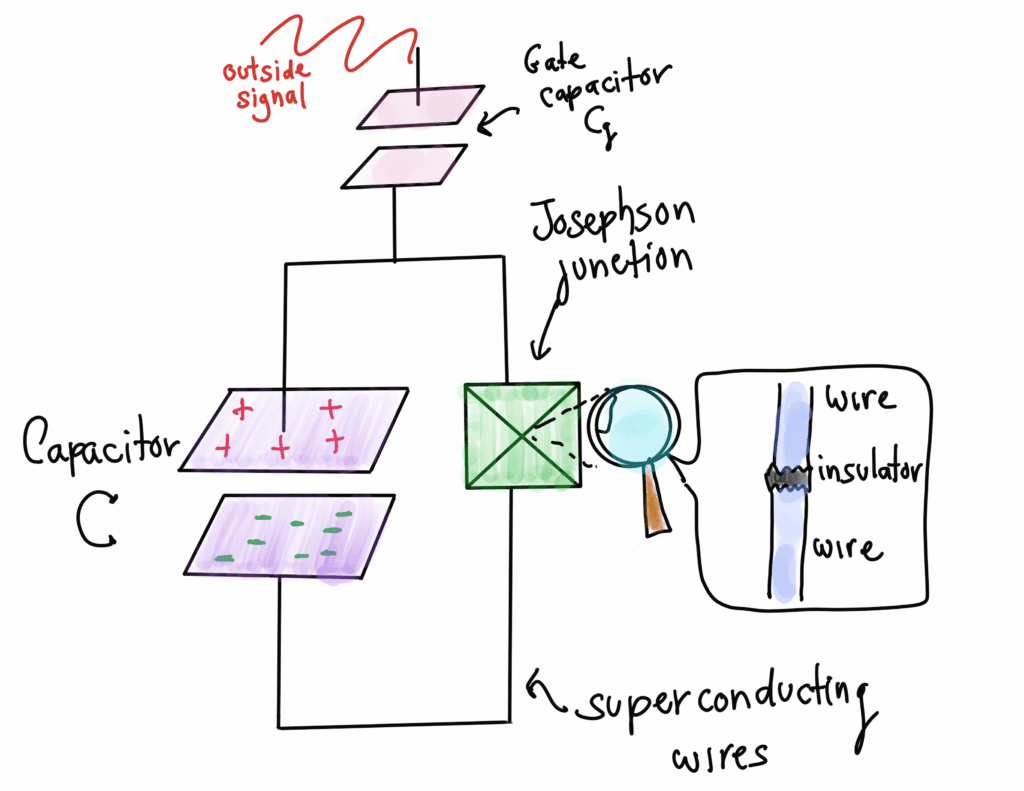
Diagram of a transmon qubit. This superconducting qubit behaves like an artificial atom with unevenly spaced energy levels. Credit to Alvaro Ballon [2].
Measuring the Qubit’s State
After fabricating a qubit, the next challenge is measuring its state reliably. In the abstract, measuring a qubit means distinguishing whether it is in state |0⟩ , state |1⟩ , or some superposition (which will collapse to either |0⟩ or |1⟩ upon measurement). Due to the incredibly fragile nature of qubits, you can’t just directly probe the qubit without disturbing it; instead, the typical approach is an indirect measurement that preserves the qubit’s information long enough to get a reading.
🔦 To measure something, we always have to interact with it in one way or another. Even the least invasive form of measurement is still a form of interaction. In everyday experience, we get to know objects by touching, opening, smelling them, and more. The least impactful approach would be to simply observe the object—arguably nothing changes on any macroscopic object when we visually inspect it. However, we’re still interacting with it via photons that bounce off the object and hit our eyes, allowing us to see and experience it. When objects become so small and sensitive that even a single photon changes their state, measurement becomes complicated. For reading the state of qubits, scientists employ something similar to looking at them: they use photons to probe and then analyze the properties of the bounced-back photons using lab instruments instead of their eyes.
The common method is to couple the qubit to a device called a readout resonator or a cavity, which is essentially a circuit that can store and transmit microwaves of a certain frequency.
To perform a measurement, a pulse of microwave light is sent into the cavity at a frequency that the cavity readily lets through (let’s call it cavity frequency). This probe frequency is chosen carefully to be different from the qubit’s transition frequency – this difference is called a detuning
Detuning =\Delta=\omega_{cavity}-\omega_{qubit},
so that the qubit itself will not absorb these photons. In other words, the measurement photons are not the right energy to flip the qubit; they just bounce off.
Even though the qubit does not absorb the probe photons, it does influence them. If the qubit is in state |0⟩ or |1⟩ , it will slightly change the electromagnetic properties of the cavity. This causes the probe microwaves to be scattered in a slightly different way depending on the qubit’s state [2].
By using sensitive electronics to detect these changes in the outgoing microwave signal, we can infer the qubit’s state without ever directly changing the qubit’s state. The measurement is gentle (ideally, it doesn’t disturb the qubit’s state until the interaction provides enough information), and it yields the outcome effectively as “qubit was |0⟩ ” or “qubit was |1⟩ ” with high probability.
Applying Single- and Two-Qubit Gates
Now that we have a working qubit and a way to measure it, the remaining piece is being able to control the qubit’s state arbitrarily – that is, to apply the quantum gates. In superconducting hardware, gates are implemented by carefully timed light pulses (often microwave signals) sent into the circuit. These control pulses nudge the qubit’s state in a precise way, as we’ll see.
For a single qubit, any arbitrary rotation of the state on the Bloch sphere can be achieved using microwave pulses. The basic idea is analogous to resonant excitation in physics: if we apply an oscillating electromagnetic field (a microwave pulse) at the qubit’s resonant frequency (the frequency corresponding to the energy gap between |0⟩ and |1⟩ ), the qubit state will undergo Rabi oscillations. By tuning the duration and strength of the pulse, we can rotate the qubit’s state vector by a desired angle in the Bloch sphere. For example, a short pulse of the right length can produce a 90° rotation (taking |0⟩ to an equal superposition of |0⟩ and |1⟩ ), while a longer pulse (twice as long) can produce a 180° rotation, which is equivalent to the NOT gate flipping |0⟩ →|1⟩ .
By combining pulses with different phases and durations, we can realize any single-qubit gate we want.
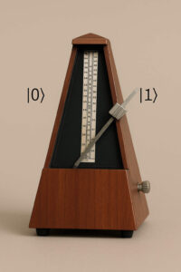
One key difference that must be highlighted is between coherent light and single photons. When considering the artificial atom system described above, sending light with the correct resonant frequency using a single photon or an incoherent ensemble of photons would simply promote the atom to the excited energy level (the one where we encoded state |1⟩ ). However, for coherent light—the type used to implement single-qubit gates—the effect is not a one-way promotion but rather a continuous oscillation between the |0⟩ ground state and the |1⟩ excited one.
We could imagine a metronome with the moving joint pointing to the “current” quantum state—on one side there is the state |0⟩ , on the other the state |1⟩ , and in between, linear combinations of the two. By shining coherent light, the metronome starts to oscillate for as long as the pulse is on, and stops in the exact position it’s in when the pulse stops. If one can precisely time the duration of the pulse, the state of the qubit can be controlled readily.
Single-qubit gates alone are not enough for universal quantum computation; we also need two-qubit gates that entangle qubits in particular at least a single two-qubit gate. In hardware terms, this means we need some way for two qubits to interact with each other in a controlled fashion.
One straightforward method is to connect the qubits via a circuit element like a capacitor. For instance, if two transmon qubits are placed on the chip near each other, a coupling capacitor between them will allow their states to influence each other. This coupling effectively creates a joint system where the two qubits’ energies become linked.
When two qubits are coupled as described above, one common entangling operation that naturally arises is the iSWAP gate. In an iSWAP, if one qubit is in |1⟩ and the other in |0⟩ , the gate will swap them (so the first becomes |0⟩ and the second |1⟩ ) and add a certain phase – it’s an entangling swap of excitations. In a capacitively coupled pair of identical qubits, if we allow them to interact for the right amount of time, they effectively undergo an iSWAP operation [2].
Returning to the previous metronome example, we could think of two-qubit gates as placing two independent metronomes on a shared platform. If one were to place two metronomes (or pendulums) on a platform that can move, the two will eventually synchronize (or anti-synchronize) following the effect called synchronization or more specifically Huygens’ synchronization of pendulum clocks.
⛵ In the 17th century, Dutch scientist Christiaan Huygens was confined to his bed with illness when he observed a curious phenomenon: two pendulum clocks hanging on the same support began ticking in perfect opposition—when one swung left, the other swung right—despite being started at different times. He had discovered what we now call synchronization: tiny vibrations traveling through the support gradually coupled the clocks’ motions until they locked into a shared rhythm. Huygens had invented the pendulum clock to address one of his era’s greatest challenges: determining longitude at sea. While sailors could establish latitude by observing the stars, they couldn’t fix their east–west position without precise timekeeping. A reliable clock was as essential as a compass for navigation. Unfortunately, pendulum clocks proved ineffective on ships, where the rolling waves disrupted their regular swinging [3].
For our two-qubit gate, we can think of the interaction between qubits as similar to allowing the shared platform of two metronomes to move. If the qubits interact for a specific duration, they begin to share their quantum states. By precisely controlling the interaction time, we can achieve the desired influence between the two qubits.
Finally, while this hardware representation is fascinating, it is more complicated to grasp. Quantum mechanics and algorithms often become so complex that relying on the abstraction of linear algebra becomes not only useful but necessary.
[1] https://arxiv.org/abs/quant-ph/0002077
[2] https://pennylane.ai/qml/demos/tutorial_sc_qubits
[3] https://www.youtube.com/watch?v=t-_VPRCtiUg
RELATED
Posts

28
May
The paradox of Intellectual Property in Deep tech
Can commercial advantage and scientific research coexist?
In late January 1987, a small group of physicists knew something the rest of the world did not. They had found a ceramic material that became superconducting at 93 kelvin, a temperature high enough...

17
Oct
Quantum Might Be The Solution to GPS Denial
Quantum sensing has shown promising results in GPS-free navigation

27
Sep
Quantum Computing and Environmental Sustainability
Quantum computing may look energy-hungry, yet its speed, chemistry breakthroughs, and reversible logic hint at a future of truly sustainable computing.

15
May
Qubits technologies
The competing technologies in the run for a Fault-Tolerant Quantum Computer

27
Feb
Microsoft Unveils Majorana 1: The First Quantum Processor with Topological Qubits
Discover Majorana 1, Microsoft's first quantum processor based on topological qubits. A breakthrough in quantum computing with the potential to solve large-scale industrial problems sooner than expected.